Learning a synthetic spike pattern

The core MNESIS experiment: a recurrent HD-SNN - one shared lin readout over the num_delay-wide spiking-history window plus one leaky integrate-and-fire (LIF) neuron per output unit, i.e. heterogeneous synaptic delays folded into delay-tap weights - must memorise a synthetic spiking motif by re-playing it from a brief trigger.

Notebook summary

Pipeline

1. Instantiate Params and the StochasticSpikingPattern generator (cf. notebook 10).

2. Analytic initialisation of net.lin.weight by regressing the target on its own sliding 41-ms windows (update_weight -> get_W_init, with LIF deconvolution and Moore-Penrose pseudo-inverse).

3. Baseline retrieval: forward pass from the trigger, scored on the evoked window.

4. Supervised learning of the same readout (learn_model driven by a F1-score loss).

5. Post-learning evaluation + weight histograms (sparsity signature).

Main outputs

• caches ../cached_data/<datetag>_init.pth (analytic init) and <datetag>_vanilla.pth (trained), each guarded by a .lock sentinel against concurrent runs;

• figures pattern.pdf, target_init.pdf, target.pdf (rasters); the weight histograms histogram_log / histogram_loglog are display-only (figpath=None).

Notes

• Baseline (analytic init) and trained scores are printed globally and motif by motif. The mean F1 is capped by the motifs that contain a gap of num_delay silent ms (motifs 3, 9, 11 and 12 for seed=2026): an empty window evokes no current, so their replay stops at the gap whatever the weights. The other failures are over-active replays, in which another motif, ignited by the spontaneous pad, is replayed alongside the correct one (paper, Sec. 3.1).

# Shared machinery from mnesis_boilerplate; the algorithm (HD_SNN) and the pattern
# generator (StochasticSpikingPattern) from mnesis_chains. Notebooks remain import-only.
from mnesis_boilerplate import torch, np, plt, splt, data_cache, cache_lock, figpath, RECOMPUTE, DEBUG, Params
from mnesis_boilerplate import printfig, get_scores, normalsize
from mnesis_chains import StochasticSpikingPattern, HD_SNN
# RECOMPUTE = True

datetag = '2026-09-07'
Using device: mps

if DEBUG > 1:
    %whos

Parameters

Params (mnesis_boilerplate.py) is the authoritative hyperparameter source

opt = Params()
opt

Params(datetag='2026-09-07', N_neuron=1024, num_delay=41, N_pattern=16, N_time=1000, N_pretime=50, p_A=0.00016, p_flip=0.01, seed=2026, lif_beta=0.7, lif_threshold=0.75, learn_beta=False, learn_threshold=False, do_pinv=True, do_deconv=True, num_epochs=256, num_warmup_epochs=16, base_lr=0.04, final_lr=0.0004, delta1=0.003, delta2=1e-05, dropout=0.6, alpha_surrogate=5.0, surrogate_name='FastSigmoid', loss_name='SpikeF1scoreLoss', reset_mechanism='zero', optimizer='adadelta', verbose=False, fig_width=15.92, phi=1.61803, fig_height=9.839125356142963, N_time_show=1000, N_neuron_show=1024, i_pattern=1, N_scan=14, N_cv=11)

group	value	meaning
topology	N_neuron=1024	presynaptic inputs / neurons forming one SM
topology	num_delay=41	width (ms) of the spiking-history (SM) window
topology	N_pattern=16	number of memorised motifs
topology	N_time=1000	duration (ms) of each motif
topology	N_pretime=50	spontaneous-activity pad before the trigger
input	p_A=1.6e-4	Bernoulli rate of the target (spikes/neuron/ms)
input	p_flip=0.01	balanced-flip rate of each training realisation
LIF	lif_beta=0.7, lif_threshold=0.75	decay / threshold, frozen (learn_*=False)
learning	adadelta, SpikeF1scoreLoss, dropout=0.6	optimiser / objective / regularisation
learning	num_epochs=256, warmup 16, LR 40 -> 0.4 mLR	cosine schedule

The two prints below sanity-check the sparsity (~164 spikes per motif, ~6.7 per 41-ms window) and the membrane time constant tau = -1/ln(beta) ~ 2.8 ms.

print(f'Spikes in one target {opt.p_A * opt.N_neuron * opt.N_time:.1f},  in a SM window {opt.p_A * opt.N_neuron * opt.num_delay:.1f}')

Spikes in one target 163.8,  in a SM window 6.7

print(f'for a value {opt.lif_beta=:.1f}, the time constant is {- 1 / np.log(opt.lif_beta):.1f} steps')

for a value opt.lif_beta=0.7, the time constant is 2.8 steps

Analytic initialisation of the readout

HD_SNN.get_W_init (called via update_weight) computes a least-squares fit of the target onto its own history: each time bin is predicted from the flattened num_delay x N_neuron sliding window of preceding spikes - the heterogeneity of synaptic delays is made explicit as delay-tap columns of one weight matrix.

• do_deconv=True: the target is first LIF-deconvolved (target - beta * roll(target, 1)) so the regression predicts the input current rather than the filtered spikes;

• do_pinv=True: Moore-Penrose pseudo-inverse (SVD on CPU); False switches to a Hebbian cross-correlation rule.

The result is cached as <datetag>_init.pth with the standard file-locking protocol: a .lock sentinel is created before computing and removed after, so concurrent notebooks never read a half-written file; RECOMPUTE=True deletes data + lock to force a redo.

# Constructing HD_SNN also initialises the (frozen) pattern generator; the analytic
# initialisation is then cached/recovered under a .lock sentinel.
hd = HD_SNN(opt, StochasticSpikingPattern())
hd.net.to(hd.opt.device)

model_init_filename = data_cache / f"{hd.opt.datetag}_init.pth"
lock_init_filename = model_init_filename.with_suffix('.lock')
if RECOMPUTE:
    model_init_filename.unlink(missing_ok=True) # FORCING RECOMPUTE
    lock_init_filename.unlink(missing_ok=True) # FORCING RECOMPUTE
try:
    model_state_dict = torch.load(model_init_filename, map_location=torch.device(hd.opt.device))
    hd.net.load_state_dict(model_state_dict)
    lock_init_filename.unlink(missing_ok=True) # in case the lock file was not unlinked
    print(f"Model weights loaded from {model_init_filename}") # Add a log message
except FileNotFoundError:
    with cache_lock(model_init_filename) as acquired:
        if acquired:
            print(f"Init file not found: {model_init_filename}, inititializing the new model.")
            ##################
            hd.update_weight()
            ##################
            torch.save(hd.net.state_dict(), model_init_filename)
        else:
            print(f"Model file is locked: {lock_init_filename}, passing.")
# in both branches: a fresh module is in train mode, and dropout (0.6) would silence the replay
hd.net.eval()

Model weights loaded from ../cached_data/2026-09-07_init.pth

Sequential(
  (lin): Linear(in_features=41984, out_features=1024, bias=False)
  (dropout): Dropout(p=0.6, inplace=False)
  (lif): Leaky()
)

Baseline retrieval from the analytic initialisation

Trigger protocol (get_input_spikes): N_pretime=50 ms of spontaneous Bernoulli(p_A) activity, then the first num_delay=41 ms of a noisy realisation of the motif (pattern_object(seed=...), balanced flips at p_flip) as the trigger; the remainder of the input raster is zero. Recurrent dynamics must re-emit the stored motif.

Evoked window - the comparison convention used by every retrieval notebook: spikes[:, :, N_pretime+num_delay : N_time+N_pretime] vs frozen_target[:, :, num_delay:] (both of length N_time - num_delay): a trigger ending at bin N_pretime+num_delay must evoke the target from its bin num_delay onwards. The reference is always the noise-free frozen_target, never the realisation used as the trigger.

# target: the frozen motif; cue: the noisy realisation whose first num_delay ms
# form the trigger. target_full: target shifted right by N_pretime so its timeline matches that of input_spikes;
# forward_pass returns (current, membrane, spikes) over the padded time axis.

with torch.no_grad():
    target = hd.pattern_object.frozen_target # noise-free reference, scored against
    cue = hd.pattern_object(seed=hd.opt.seed) # seeded noisy realisation, provides the trigger
    target_full = torch.nn.functional.pad(target, (opt.N_pretime, opt.N_pretime))
    input_spikes = hd.get_input_spikes(target=cue, seed=hd.opt.seed)
    current, mem, spikes = hd.forward_pass(input_spikes)
current.min().item(), current.mean().item(), current.max().item()

(-0.9999959468841553, 4.3373493099352345e-05, 1.022775650024414)

# Score only the evoked window (aligned slices of length N_time - num_delay).

with torch.no_grad():
    spikes_evoked = spikes[:, :, (hd.opt.N_pretime+hd.opt.num_delay):(hd.opt.N_time+hd.opt.N_pretime)]
    target_evoked = target[:, :, hd.opt.num_delay:]
    precision, recall, f1_score = get_scores(spikes_evoked, target_evoked)
    print(f'precision = {precision:.3f}\t recall = {recall:.3f}\t f1_score = {f1_score:.3f} ')
    # Per-motif scores (axis 0 = motif): the global score pools all spikes and can hide a motif that fails.
    for i_pattern in range(target_evoked.shape[0]):
        precision_i, recall_i, f1_score_i = get_scores(spikes_evoked[i_pattern], target_evoked[i_pattern])
        print(f'motif {i_pattern:2d}: precision = {precision_i:.3f}\t recall = {recall_i:.3f}\t f1_score = {f1_score_i:.3f} ')

precision = 0.835        recall = 0.825  f1_score = 0.830
motif  0: precision = 0.546      recall = 1.000  f1_score = 0.706
motif  1: precision = 1.000      recall = 1.000  f1_score = 1.000
motif  2: precision = 1.000      recall = 1.000  f1_score = 1.000
motif  3: precision = 1.000      recall = 0.175  f1_score = 0.298
motif  4: precision = 0.586      recall = 1.000  f1_score = 0.739
motif  5: precision = 1.000      recall = 1.000  f1_score = 1.000
motif  6: precision = 1.000      recall = 1.000  f1_score = 1.000
motif  7: precision = 1.000      recall = 1.000  f1_score = 1.000
motif  8: precision = 1.000      recall = 1.000  f1_score = 1.000
motif  9: precision = 1.000      recall = 0.221  f1_score = 0.362
motif 10: precision = 0.653      recall = 1.000  f1_score = 0.790
motif 11: precision = 1.000      recall = 0.294  f1_score = 0.454
motif 12: precision = 0.462      recall = 0.564  f1_score = 0.508
motif 13: precision = 1.000      recall = 1.000  f1_score = 1.000
motif 14: precision = 1.000      recall = 1.000  f1_score = 1.000
motif 15: precision = 1.000      recall = 1.000  f1_score = 1.000

Raster legend (trigger vs. target)

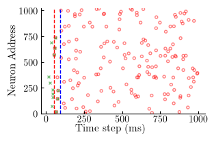
Open red o = the frozen target, padded by N_pretime on both sides so it aligns with the input timeline; green x = the trigger (spontaneous pad + first num_delay ms of the noisy realisation). Red/blue dashed verticals mark N_pretime (trigger onset) and N_pretime + num_delay (start of the evoked window).

All the rasters of this notebook show the motif opt.i_pattern = 1 (0-based), the second of the N_pattern = 16 motifs (Figure fig:target of the paper): it is numbered 2, in bold, in the retrieval figure of notebook 13.

# Drawn at its printed size: half of \textwidth (A4, 1 in margins), golden ratio, as
# tex/tikz_snntorch.pdf, so both panels of fig:model share the same height at scale 1.
# The axes are then pinned on the rows of that diagram (fractions of its height): top
# of the axes on the output arrow tips, x axis on the bottom of the X[t] boxes, x label
# on the baseline of the "t = 0" labels. bbox=None keeps that exact geometry.
textwidth = 15.92  # (cm)
tikz_border = 2 / 72.27 * 2.54  # standalone border (cm)
tikz_y0, tikz_y1 = -3.427 - tikz_border, 3.627 + tikz_border  # bounding box (cm)
tikz_frac = lambda y: (y - tikz_y0) / (tikz_y1 - tikz_y0)
# the diagram is printed at tikz_scale of its natural width (11.5 cm plus the borders), and its
# fonts are enlarged by 1 / tikz_scale so that they print at the text size, as this raster
tikz_scale = 0.49 * textwidth / (11.5 + 2 * tikz_border)
# "t = 0" is a \papernormalsize node at y = -3.15 cm, centred on digits about 0.645 em high
t_baseline = -3.15 - 0.645 * normalsize / tikz_scale / 72.27 * 2.54 / 2  # (cm)

fig, ax = plt.subplots()
splt.raster(target_full[opt.i_pattern, :opt.N_neuron_show, :opt.N_time_show].T, ax, s=8, facecolor='none', edgecolor='red',  marker='o', alpha=.5)
splt.raster(input_spikes[opt.i_pattern, :opt.N_neuron_show, :opt.N_time_show].T, ax, s=8, c="green", marker='x', alpha=.5)
ax.vlines([opt.N_pretime], 0, opt.N_neuron_show, 'r', ls='--')
ax.vlines([opt.N_pretime+opt.num_delay], 0, opt.N_neuron_show, 'b', ls='--')
ax.set_xlabel("Time step (ms)", va='baseline')
ax.xaxis.set_label_coords(0.5, tikz_frac(t_baseline), transform=fig.transFigure)
ax.tick_params(axis='x', pad=1.0)
ax.set_ylabel("Neuron Address", labelpad=1.5)
ax.set_ylim(-1., opt.N_neuron_show + 1.)
fig.subplots_adjust(top=tikz_frac(2.45 + 0.45 + 0.6), bottom=tikz_frac(-1.9 - 0.45), left=0.17, right=0.95)
printfig(fig, 'pattern', fig_width=0.49*textwidth, fig_height=0.49*textwidth/opt.phi, figpath=figpath, bbox=None, layout=None)
spikes.shape, spikes[opt.i_pattern, :opt.N_neuron_show, :opt.N_time_show].sum().item(), target[opt.i_pattern, :, :].sum().item()

Saving as ../figures/pattern.pdf
Saving as ../figures/pattern.png
Saving as ../figures/pattern.svg

(torch.Size([16, 1024, 1100]), 155.0, 165.0)

Raster legend (adds the evoked response)

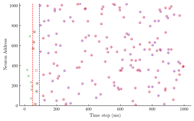
Blue + = spikes re-emitted by the network in the evoked window. Blue aligning with red o is a correct retrieval; blue without red = false positives (precision loss), red without blue = misses (recall loss).

fig, ax = plt.subplots()
splt.raster(spikes[opt.i_pattern, :opt.N_neuron_show, :opt.N_time_show].T, ax, s=25, c="blue", marker='+', alpha=.5)
splt.raster(target_full[opt.i_pattern, :opt.N_neuron_show, :opt.N_time_show].T, ax, s=25, facecolor='none', edgecolor='red',  marker='o', alpha=.5)
splt.raster(input_spikes[opt.i_pattern, :opt.N_neuron_show, :opt.N_time_show].T, ax, s=25, c="green", marker='x', alpha=.5)
ax.vlines([opt.N_pretime], 0, opt.N_neuron_show, 'r', ls='--')
ax.vlines([opt.N_pretime+opt.num_delay], 0, opt.N_neuron_show, 'b', ls='--')
ax.set_xlabel("Time step (ms)")
ax.set_ylabel("Neuron Address")
ax.set_ylim(-1., opt.N_neuron_show + 1.)
printfig(fig, 'target_init', fig_width=opt.fig_width, fig_height=opt.fig_height, figpath=figpath)
spikes.shape, spikes[opt.i_pattern, :opt.N_neuron_show, :opt.N_time_show].sum().item(), target[opt.i_pattern, :, :].sum().item()

Saving as ../figures/target_init.pdf
Saving as ../figures/target_init.png
Saving as ../figures/target_init.svg

(torch.Size([16, 1024, 1100]), 155.0, 165.0)

Supervised learning of the readout

learn_model refines net.lin.weight (the only trainable tensor) with:

• loss SpikeF1scoreLoss = 1 - F1, computed only on the evoked window ([N_pretime+num_delay : N_time+N_pretime] vs target[:, num_delay:]);

• optimiser adadelta (rho = 1 - delta1 = 0.997) and a cosine LR schedule with a 16-epoch warmup, decaying base_lr=40 mLR to final_lr=0.4 mLR;

• dropout 0.6 on the post-synaptic current, and a fresh stochastic realisation of the frozen pattern at every epoch (pattern_object(seed=...)) - data augmentation against memorising one exact realisation;

• per-epoch metrics on a second held-out realisation used as the trigger, scored against the frozen pattern and logged every num_epochs // 64 epochs; all realisations are seeded from seed, so a run is reproducible.

Same .pth + .lock caching as the init stage.

model_filename = data_cache / f"{hd.opt.datetag}_vanilla.pth"
lock_filename = model_filename.with_suffix('.lock')
if RECOMPUTE:
    model_filename.unlink(missing_ok=True) # FORCING RECOMPUTE
    lock_filename.unlink(missing_ok=True) # FORCING RECOMPUTE
try:
    model_state_dict = torch.load(model_filename, map_location=torch.device(hd.opt.device))
    hd.net.load_state_dict(model_state_dict)
    lock_filename.unlink(missing_ok=True) # in case the lock file was not unlinked
    print(f"Model weights loaded from {model_filename}") # Add a log message
except FileNotFoundError:
    with cache_lock(model_filename) as acquired:
        if acquired:
            print(f"Model file not found: {model_filename}, training a new model.")
             ##################
            hd.learn_model()
             ##################
            torch.save(hd.net.state_dict(), model_filename)
        else:
            print(f"Model file is locked: {lock_filename}, passing.")
hd.net.eval()

Model weights loaded from ../cached_data/2026-09-07_vanilla.pth

Sequential(
  (lin): Linear(in_features=41984, out_features=1024, bias=False)
  (dropout): Dropout(p=0.6, inplace=False)
  (lif): Leaky()
)

Post-learning evaluation

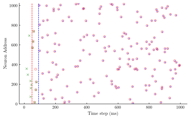
Same trigger protocol (same seeded realisation), evoked-window slices and frozen reference as the baseline: compare with the analytic-init scores printed above to quantify what supervised refinement adds. eval() turns dropout off, so the pass is deterministic.

with torch.no_grad():
    target_full = torch.nn.functional.pad(target, (opt.N_pretime, opt.N_pretime))
    input_spikes = hd.get_input_spikes(target=cue, seed=hd.opt.seed)
    _, _, spikes = hd.forward_pass(input_spikes)
    spikes_evoked = spikes[:, :, (hd.opt.N_pretime+hd.opt.num_delay):(hd.opt.N_time+hd.opt.N_pretime)]
    target_evoked = target[:, :, hd.opt.num_delay:]

    precision, recall, f1_score = get_scores(spikes_evoked, target_evoked)
    print(f'precision = {precision:.3f}\t recall = {recall:.3f}\t f1_score = {f1_score:.3f} ')
    # Per-motif scores (axis 0 = motif): the global score pools all spikes and can hide a motif that fails.
    for i_pattern in range(target_evoked.shape[0]):
        precision_i, recall_i, f1_score_i = get_scores(spikes_evoked[i_pattern], target_evoked[i_pattern])
        print(f'motif {i_pattern:2d}: precision = {precision_i:.3f}\t recall = {recall_i:.3f}\t f1_score = {f1_score_i:.3f} ')

precision = 0.835        recall = 0.825  f1_score = 0.830
motif  0: precision = 0.546      recall = 1.000  f1_score = 0.706
motif  1: precision = 1.000      recall = 1.000  f1_score = 1.000
motif  2: precision = 1.000      recall = 1.000  f1_score = 1.000
motif  3: precision = 1.000      recall = 0.175  f1_score = 0.298
motif  4: precision = 0.586      recall = 1.000  f1_score = 0.739
motif  5: precision = 1.000      recall = 1.000  f1_score = 1.000
motif  6: precision = 1.000      recall = 1.000  f1_score = 1.000
motif  7: precision = 1.000      recall = 1.000  f1_score = 1.000
motif  8: precision = 1.000      recall = 1.000  f1_score = 1.000
motif  9: precision = 1.000      recall = 0.221  f1_score = 0.362
motif 10: precision = 0.653      recall = 1.000  f1_score = 0.790
motif 11: precision = 1.000      recall = 0.294  f1_score = 0.454
motif 12: precision = 0.462      recall = 0.564  f1_score = 0.508
motif 13: precision = 1.000      recall = 1.000  f1_score = 1.000
motif 14: precision = 1.000      recall = 1.000  f1_score = 1.000
motif 15: precision = 1.000      recall = 1.000  f1_score = 1.000

fig, ax = plt.subplots()
splt.raster(spikes[opt.i_pattern, :opt.N_neuron_show, :opt.N_time_show].T, ax, s=25, c="blue", marker='+', alpha=.5)
splt.raster(target_full[opt.i_pattern, :opt.N_neuron_show, :opt.N_time_show].T, ax, s=25, facecolor='none', edgecolor='red',  marker='o', alpha=.5)
splt.raster(input_spikes[opt.i_pattern, :opt.N_neuron_show, :opt.N_time_show].T, ax, s=25, c="green", marker='x', alpha=.5)
ax.vlines([opt.N_pretime], 0, opt.N_neuron_show, 'r', ls='--')
ax.vlines([opt.N_pretime+opt.num_delay], 0, opt.N_neuron_show, 'b', ls='--')
ax.set_xlabel("Time step (ms)")
ax.set_ylabel("Neuron Address")
ax.set_ylim(-1., opt.N_neuron_show + 1.)
printfig(fig, 'target', fig_width=opt.fig_width, fig_height=opt.fig_height, figpath=figpath)
spikes.shape, spikes[opt.i_pattern, :, :].sum().item(), target[opt.i_pattern, :, :].sum().item()

Saving as ../figures/target.pdf
Saving as ../figures/target.png
Saving as ../figures/target.svg

(torch.Size([16, 1024, 1100]), 158.0, 165.0)

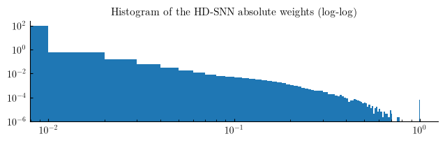
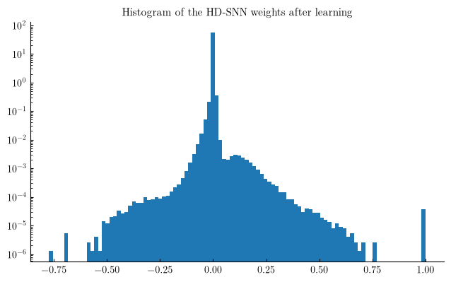
Weight histograms: sparsity signature

100-bin density histograms of the trained net.lin.weight (41984 x 1024 = one delay tap x one post-synaptic neuron), on log (and log-log) scales. A tall peak near zero with heavy tails = a sparse code: few strong, selective synapses carry each memory.

# hd.net.lin.bias.cpu().detach().numpy()
fig, ax = plt.subplots()
ax.hist(hd.net.lin.weight.cpu().detach().numpy().ravel(), bins=100, density=True) # pyright: ignore[reportCallIssue, reportAttributeAccessIssue]
ax.set_title(f"Histogram of the HD-SNN weights after learning")
ax.set_yscale('log')
printfig(fig, 'histogram_log', fig_width=opt.fig_width, fig_height=opt.fig_height, figpath=figpath)

Saving as ../figures/histogram_log.pdf
Saving as ../figures/histogram_log.png
Saving as ../figures/histogram_log.svg

# hd.net.lin.bias.cpu().detach().numpy()
fig, ax = plt.subplots()
ax.hist(np.abs(hd.net.lin.weight.cpu().detach().numpy().ravel()), bins=100, density=True) # pyright: ignore[reportCallIssue, reportAttributeAccessIssue]
ax.set_title(f"Histogram of the HD-SNN absolute weights (log-log)")
ax.set_yscale('log')
ax.set_xscale('log')
printfig(fig, 'histogram_loglog', fig_width=opt.fig_width, fig_height=opt.fig_height/2, figpath=None)